

Guide


- SmartDalton™ only works on Windows Operating System. Please make sure you have Windows 7 (or later versions) installed in your computer.
- It is required that your computer has Java 8 – 64 bit (minimum). Here is the link for your convenience if there is a need to install: https://java.com/en/download/manual.jsp

- To use SmartDalton™, the computer screen resolution has to be set to at least Full HD – 1920 x 1080 pixels.
- Select New Data button to load the *.CDF sample data. This will load up the TIC profile of the sample data

- Select Auto Cut button to perform peak-picking function.

- Select Data Source Type button to identify the brand of GC-MS equipment used for data collection. Available options include Agilent, Shimadzu and Generic (for all other brands).
- Select Cut Sensitivity button to determine the sensitivity of the peak-picking function. Available options include Normal, High and Ultra. The High and Ultra modes enable the detection of trace and ultra-trace components, respectively.
- The upper and lower limits of TIC time and m/z range can be modified for peak-picking if required. Leave the values as it is to analyze the entire TIC time and m/z range.
- Specific m/z channels can be omitted from analysis, such as m/z channels corresponding to consistent background or column bleed. Select Add or Remove to include or omit a specific m/z channel.
- Select OK to proceed with automated peak-picking.

- The following screen will appear after the peak-picking process is completed. The detected peak intervals are tabulated on the right side. Upon selection of a peak interval, the corresponding TIC plot and 3D plot of the raw data will be displayed on the lower half of the Data Processing Page.

- Select a peak interval from the table.

Note: Keyboard shortcuts are available. W to scroll up. S to scroll down. R to perform deconvolution for the particular peak interval. Ctrl+D to delete a peak interval. Note that deletion cannot be undone. - The TIC plot of the selected peak interval will be shown.
Ensure that the peak interval covers the entire TIC profile of the intended peak. Use the 3D plot to judge the suitability of the peak interval.
In order to modify the width of a peak interval, drag and highlight the intended peak interval with the mouse. Select the + and – buttons to zoom in/out. Select Save button to overwrite the original peak interval.
Select the Add button to add a new entry of peak interval into the table list without overwriting the original peak interval. The new entry will appear at the bottom of the table. Simply click the Start header of the table to rearrange the list accordingly.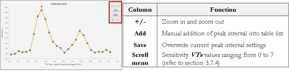
Zoom out the TIC plot to ensure that you do not accidentally leave out any peak interval. Peak intervals that are listed in the table will be color-coded in the zoom-out TIC plot (The TIC plot below consists of four peak intervals that are listed in the table). The red inverted triangles indicate the global peak apex for each peak interval.
The TIC profile in black are regions that are not included in the table, and thus will not be analyzed.
The peak picking function increases the probability of detecting trace components by representing the detected peaks in a parent-daughter relationship.
In the Ref. column of the table, a parent peak is labelled as ## while daughter peaks are labelled as ##-##.
Delete either the daughter or parent peak. To delete an entry, select the intended peak interval and press Ctrl+D. Alternatively, check the box in the Action column of the table and press the right mouse button followed by Delete All Checked Area.
- The 3D plot of the selected peak interval will also be shown.The 3D plot can be rotated by pressing the left mouse button and drag in the intended direction. The displayed 3D plot is a low-resolution plot. High-resolution 3D plot can be viewed by selecting HD Plot in 3D button.
Uncheck the 3D View/MS View to view the mass spectrum of a particular sampling point selected in the TIC plot. Select Zoom Plot for MS button to view an enlarged version.
Note:
• Use the 3D plot to improve the judgment for analysis. The axes of the 3D plot include m/z, TIC time and intensity. A unique component will have a series of peaks across numerous m/z channels.
• While SmartDalton™ is capable of analyzing multi-component peaks, users are advised to restrict a peak interval to contain approximately 2-3 components for a faster and more robust deconvolution.
Notes:
- SmartDaltonTM can be halted at any point of time. Please save the peak interval table information by selecting Save Batch File. The batch file (*.cpb) will be auto-generated in the Data Folder, which was set up in Step 3.1.
- Analysis can be resumed at a later time by selecting Open Batch File button to load the *.cpb file.

- Analysis can also be resumed by selecting Load Saved Job in the Welcome Page.
- To perform deconvolution, press and hold the Ctrl button on keyboard and select the Run button. When prompted, save the batch file in the same Data Folder. The deconvolution process may take around 30 minutes depending on the number of peak intervals analyzed.The process can be terminated by selecting Ctrl button + Terminating Run and resumed at a later time.

- The following Result Review Page will appear after the deconvolution process is completed. The deconvolution result window will show the deconvoluted component profiles. The corresponding pure mass spectrum for the selected component will be displayed in the window below.
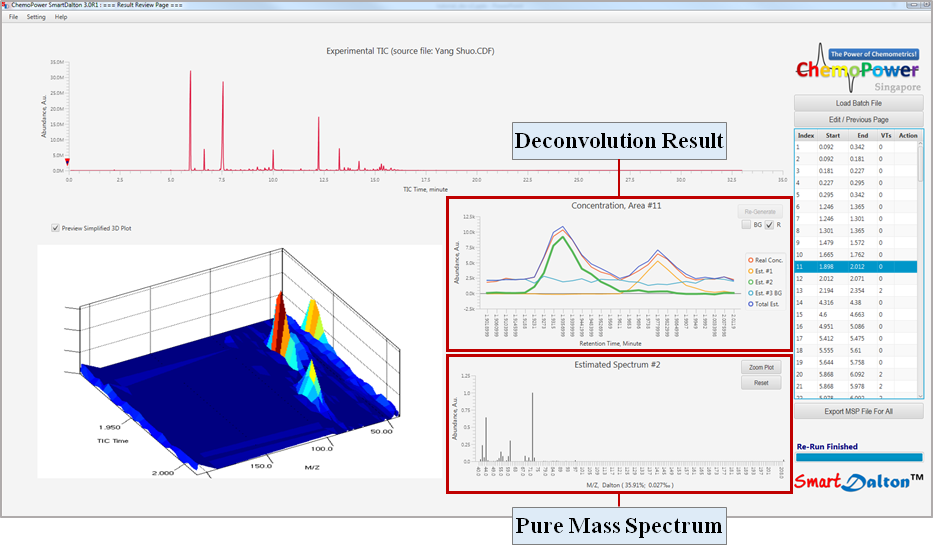
- Identify components (Est #) that are background signals.
Background signals usually have a flat profile (e.g., component Est. #3 below).
Assign a component as background signal by first selecting the component by clicking on the TIC profile or plot legend. Next, check the BG box.
A component which has been assigned as a background signal will have the code ‘BG’ embedded in the plot legend.
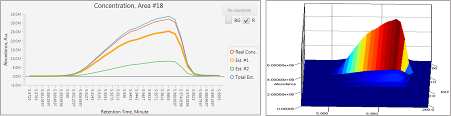
Another scenario which you may come across is seeing perfectly mirrored line, as illustrated below (Est #2 and #3 are mirror image). These lines are deemed as background signals and can be corrected. This correction will not affect or change the results of the estimated spectra.
Select one of the mirrored line and uncheck the R box to not retain the estimated component.
Select Regenerate button to correct the profiles. Remember to assign the component as background before proceeding.

- Re-run the deconvolution process if the result is not satisfactory.
Select the peak interval of interest and press R on the keyboard to re-run the deconvolution. Otherwise, right click and select Re-Run This Area.
Note:
• GC-MS data typically consists of background noise signals.
• A good overlap between the Total Est. and Rel. Conc. profiles is a good indicator of a good deconvolution result. - If there is a need to delete a peak interval, select the peak interval and press Ctrl+D on the keyboard. Please note that this action cannot be undone.
- To modify the peak interval, return to the Data Processing Page by selecting the Edit/Previous Page button.
Adjustment of peak interval width and VTs are shown in Section 3.5. Briefly, select the intended VTs and select Save button. Press R on the keyboard to preview the deconvolution result of the new VTs setting without proceeding to the Result Review Page.
Note:
• SmartDaltonTM provides an automated deconvolution solution. This function is represented as VTs=0.
• If the automated deconvolution solution is not satisfactory, users can perform a semi-automated analysis by varying the VTs from a range of 2 to 7.
• Based on the observation of the 3D plot, users are advised to input a VTs value that is close to the number of components observed in the 3D plot.
• Changes to VTs should be reflected in the table list. - The analysis of pure peak, whereby a peak interval consisting of only one unique chemical component and without a background signal, may result in unsatisfactory deconvolution due to the sensitivity of the algorithm.
To correct this, right click the peak interval from the table and select Process as Pure Peak.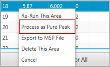
The profile will be corrected as below.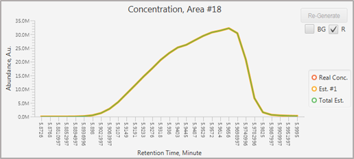
- To export the mass spectra for subsequent spectral match analysis, select Export MSP File For All button. A collated *.msp file will be generated in the Data Folder.
The *.msp file can be loaded into NIST MS Search or ChemoPower’s MoleculeDBTM for spectral match analysis.
To generate a *.msp file for a specific peak interval, right click at the peak interval and select Export to MSP File.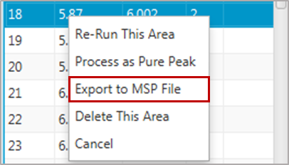
Prerequisite: You need to have the NIST Program and NIST library
Loading *.msp File into NIST Program For Head-to-Tail M/Z Spectrum Matching
1) Locate your *.msp file on your hard disk. (Please do not double-click the *.msp file, which will pop-up a “Window Installer” error message – which is not important and can be ignored)
2) Open your NIST “MS search V2.x” main program.
3) Load the *.msp file into your NIST software by clicking menu tab “File” → “Open…” to open it. (see figure as follows)

4) At pop-up window, click “Import All”.

Note: The import list will be very long and this is the reason why we do not want to include backgrounds in our analysis as they are meaningless and will save us time.(As explained in “Step-by-step SmartDaltonTM Guide” Step 11)
5) The NIST program will automatically start matching the spectra, as follows.

6) Once the matching is completed, double click each item in the list at the top left corner of the window, to check the match results.
Do “Double Click” every item to check the matching, otherwise, it will not refresh the spectrum in library.

7) Choose “Head to Tail” tab in the middle right box to compare the results.

8) Click the items in the list at the bottom left of the window to find the best head-to-tail matching results.


